Axisymmetric Fluid Filled Pipe

This example details a more complex application of the pywfe package to an axisymmetric fluid filled pipe.

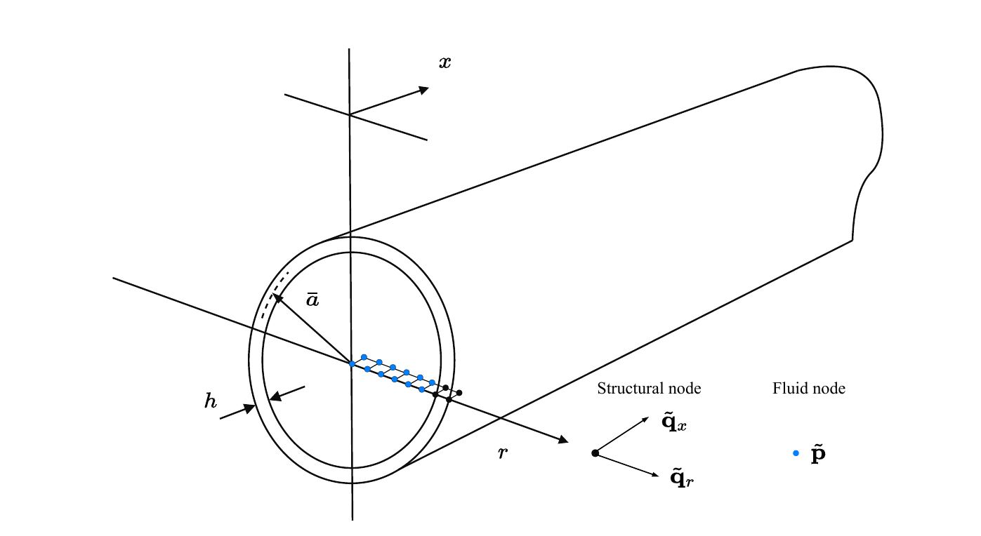
The mesh information was initially generated using COMSOL Multiphysics with cyclic symmetry. As such, the system descibes axisymmetric (otherwise known as \(n=0\)) motion. The pipe structure modelled as steel with a hysteretic loss factor of 0.1%, the inner radius is 0.2m and the outer radius is 0.21

Loading and Inspecting the Model

The pipe model in this example has been saved into the package database, and can be loaded with

import numpy as np
import pywfe
import matplotlib.pyplot as plt

model = pywfe.load("AXISYM_thick_0pt1pc_damping", source='database')

The model description, which is optionally added before saving returns:

print(model.description)

>>> WFE Segment of water filled pipe
>>>
>>> Inner radius: 20cm, Outer radius: 21cm
>>> Steel Youngs mod: 19.2e10*(1 + eta_s*i), Poissons ratio: 0.3, Steel density: 7850,
>>> Water bulk mod: 2.1e9*(1 + eta_f*i), Water density: 1000
>>>
>>> Steel loss-factor = 0.001
>>> Water loss-factor = 0
>>> maximum element size = 1cm

>>> Outer radial forcing dof index: 45

With pywfe.Model.see() the model mesh can be visualised, showing the left face of the segment. In this case, since the model is 2D and axisymmetric, the left face is a line of nodes.

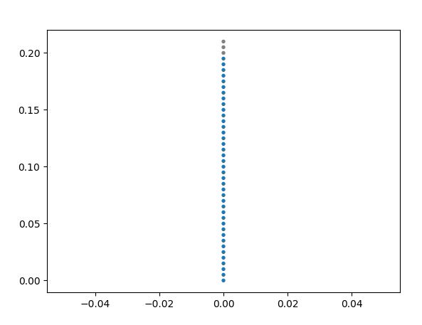
The dof attribute contains more information about the degrees of freedom. For example, print(set(model.dof['fieldvar'])) will show the unique field variables in the model which are 'u', 'w' 'p'. These are the two structural (radial and longitdunal) degrees of freedom in the pipe wall and the pressure in the pipe fluid respectively. Clicking on the nodes displayed with pywfe.Model.see() using an interactive matplotlib backend will print information about that node.

Free Wave Solutions

Dispersion Curves

As with the (Analytical Beam Example), the dispersion curves of the system can be calculated:

f_arr = np.linspace(10, 10e3, 300)

k = model.dispersion_relation(f_arr)

plt.subplot(2, 1, 1)
plt.plot(f_arr, k.real, '.')
plt.ylabel('Re(k)')
plt.ylim(0, 50)

plt.subplot(2, 1, 2)
plt.plot(f_arr, k.imag, '.')
plt.ylabel('Im(k)')
plt.ylim(0, -50)

plt.xlabel('Frequency (Hz)')

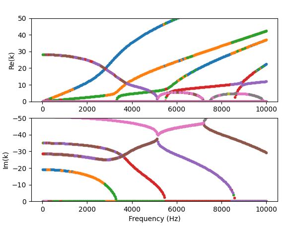
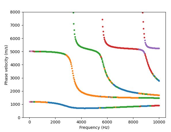
The solutions wavenumber solutions are not sorted, and so are plotted as a scatter plot. The phase velocity curves can also be computed with pywfe.Model.phase_velocity(). In this case, the wavenumbers are already computed, and the phase velocity can be calculated via its definition. Only strongly propagating modes are plotted:

k_prop = np.copy(k)
k_prop[abs(k.imag) > 0.5] = np.nan

c_p = 2*np.pi*f_arr[:, None]/k_prop

plt.plot(f_arr, c_p, '.')
plt.ylim(0, 8e3)

plt.xlabel('Frequency (Hz)')

Mode Shapes

Also of interest for the free-wave solutions are the mode shapes. These could be calculated for each frequency with pywfe.Model.generate_eigensolution(), which gives the raw eigensolution. Instead, it is convenient to use the pywfe.Model.frequency_sweep() method, which allows many different frequency dependent quantities to be solved together with each frequency step. The positive-going wavenumbers and mode shapes are requested for the frequency sweep, and are stored in a dictionary.

sweep_result = model.frequency_sweep(
f_arr, quantities=['wavenumbers', 'phi_plus'])

NOTE: The pywfe.Model.frequency_sweep() method allows the modal assurance criterion to be used to track each mode across sufficiently fine frequency steps.

sweep_result = model.frequency_sweep(
f_arr, quantities=['wavenumbers', 'phi_plus'], mac = True)

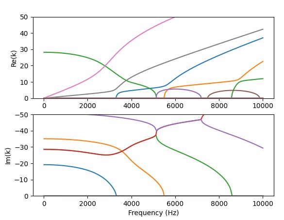
Now the dispersion relation can be plotted with continuous curves in the wavenumber domain:

plt.subplot(2, 1, 1)
plt.plot(f_arr, sweep_result['wavenumbers'].real)
plt.ylabel('Re(k)')
plt.ylim(0, 50)
plt.subplot(2, 1, 2)
plt.plot(f_arr, sweep_result['wavenumbers'].imag)
plt.ylabel('Im(k)')

plt.xlabel('Frequency (Hz)')
plt.ylim(0, -50)

The mode shapes from the frequency sweep have the shape (n. frequencies, n. dofs, n.modes).

phi = np.copy(sweep_result['phi_plus'])

print(phi.shape)
>>> (300, 94, 47)

The first half of the dof axis represents the free-wave modal displacements, and the second half the forces. We select just the displacement part of the mode shapes with

# get just the displacement component of the mode shapes by slicing down the second axis
phi_q = phi[:, :model.N//2, :]

Selecting Degrees of Freedom

The displacement mode shapes contain both the structural displacements and pressures. To separate these out, the method pywfe.Model.select_dofs() is provided. The dofs are selected by their field variable with:

struc_dof = model.select_dofs(fieldvar=['u', 'w'])
fluid_dof = model.select_dofs(fieldvar='p')

which returns a reduced dof dictionary for each selection. To select the part the corresponding part of the mode shape array, pywfe.Model.dof_to_indices() is used:

fluid_dof_indices = model.dof_to_indices(fluid_dof)
phi_p = phi_q[fluid_dof_indices]

phi_p now represents the pressure mode shapes.

Mode Sorting

Before plotting the mode shapes, There is one more useful function for sorting the free-wave solutions. The function pywfe.sort_wavenumbers() can be used on a wavenumber solution to produce sorted indices for modes according to their order of cut-on.

The free-wave solutions can now be sorted along the modal axis with

sorted_mode_indices = pywfe.sort_wavenumbers(sweep_result['wavenumbers'])

k_sorted = np.copy(sweep_result['wavenumbers'])[..., sorted_mode_indices]
phi_p_sorted = np.copy(phi_p)[..., sorted_mode_indices]

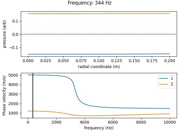
np.copy is used to keep the sorted and unsorted solutions separate to avoid confusion. The pressure mode shapes for the first two propagating modes are now plotted at a low frequency:

radial_coord = fluid_dof['coord'][1]
frequency_index = 10

for mode_index in [0, 1]:

    plt.subplot(2, 1, 1)

    plt.plot(radial_coord, phi_p_sorted[frequency_index, :, mode_index])
    plt.axhline(y=0)
    plt.xlabel('radial coordinate (m)')
    plt.ylabel('pressure (arb)')

    plt.subplot(2, 1, 2)

    plt.plot(f_arr, 2*np.pi*f_arr /
            k_sorted[..., mode_index], label=f'mode {mode_index}')
    plt.axvline(x=f_arr[frequency_index], color='black')
    plt.xlabel('frequency (Hz)')
    plt.ylabel('Phase velocity (m/s)')

plt.legend(loc='best')
plt.suptitle(f'Frequency: {f_arr[frequency_index]:.0f} Hz')
plt.tight_layout()
plt.title()

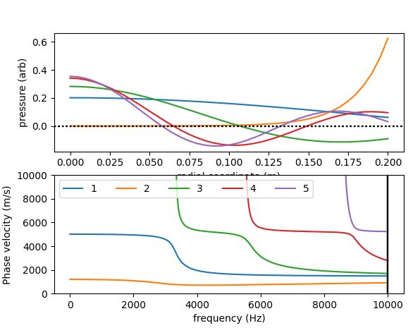
Now all 5 propagating pressure modes at the maximum frequency of interest are plotted:

frequency_index = -1

# plot only the propagating wavenumbers
k_sorted_propagating = np.copy(k_sorted)
k_sorted_propagating[abs(k_sorted.imag) > 0.5] = np.nan

for mode_index in [0, 1, 2, 3, 4]:

    plt.subplot(2, 1, 1)

    plt.plot(radial_coord, phi_p_sorted[frequency_index, :, mode_index])
    plt.axhline(y=0, color='black', linestyle=':')
    plt.xlabel('radial coordinate (m)')
    plt.ylabel('pressure (arb)')

    plt.subplot(2, 1, 2)

    plt.plot(f_arr, 2*np.pi*f_arr /
            k_sorted_propagating[..., mode_index], label=f'{mode_index + 1}')

    plt.axvline(x=f_arr[frequency_index], color='black')
    plt.xlabel('frequency (Hz)')
    plt.ylabel('Phase velocity (m/s)')

plt.subplot(2, 1, 2)
plt.ylim(0, 10e3)
plt.legend(loc='best', ncols=5)

Model Forcing

We now add a radial force to the outer pipe wall with the appropriate degree of freedom.

# add a 1 newton radial force to the outer pipe wall
model.force[45] = 1

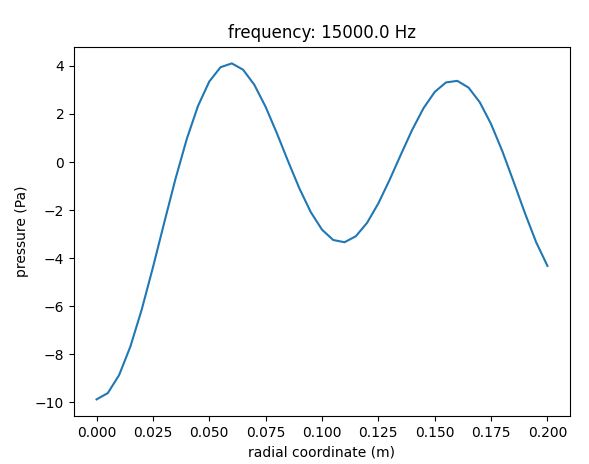
With this loading added the forced response can be calculated with a number of methods. For example, to calculate the pressure field at x=0:

# plot the pressure across the the radial coordinate at x=0
excitation_frequency = 15e3

p0 = model.displacements(f=excitation_frequency, x_r=0, dofs=fluid_dof)

plt.plot(radial_coord, p0)
plt.xlabel('radial coordinate (m)')
plt.ylabel('pressure (Pa)')
plt.title(f'frequency: {excitation_frequency} Hz')

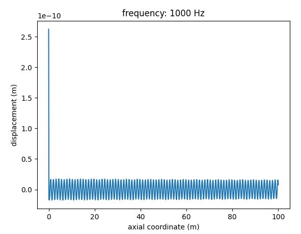
Or to calculate the radial displacement at the outer wall (the same dof at which the forcing was applied):

excitation_frequency = 1000

x_arr = np.linspace(0, 100, 1000)

u_x = model.displacements(f=excitation_frequency, x_r=x_arr, dofs=[45])

plt.plot(x_arr, u_x)
plt.xlabel('axial coordinate (m)')
plt.ylabel('displacement (m)')
plt.title(f'frequency: {excitation_frequency} Hz')

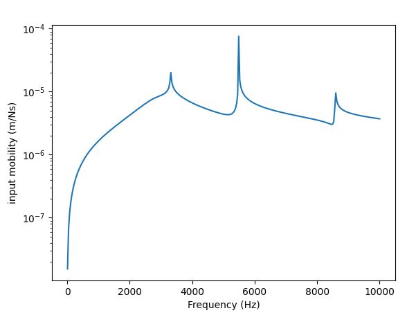
To calculate the input mobility, we use pywfe.Model.tranfer_function() at x=0 over a given frequency range with derivative=1 to return the structural velocity (the input force is 1N)

input_mobility = model.transfer_function(f_arr, x_r=0, dofs=[45], derivative=1)

plt.semilogy(f_arr, abs(input_mobility))
plt.xlabel('Frequency (Hz)')
plt.ylabel('input mobility (m/Ns)')

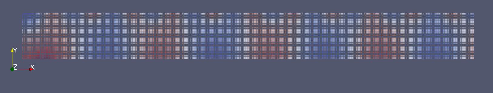
Finally, to allow easier visualisation of results without wrestling with matplotlib, a displacement/pressure field can be saved into the .vtu format for loading into ParaView. See pwfe.save_as_vtk(). Here we save the pressure field from 0-2m at an excitation frequency of 4kHz